
Part 3. Advanced Use: Replacing all generic textures with real world data and embedding the changes
Note: The NLCD Template project and all data referred to in this tutorial are available on the free NLCD Data Set download.
In this part of the tutorial, we are going to extend the changes we made in the second part to include the whole of our 1-m orthophoto, while leaving the generic texturing elsewhere. We are also going to take a quick look at enhancing the changes with the addition of walls for major buildings and then embed those changes in our project so as to prevent the original NLCD template texturing from taking precedence the next time our Rhode Island project is loaded.
1. Run VNS and select File>New from the main menu. Call your new project NLCDTutorial3 and click the Clone an Existing Project checkbox to select it.
2. Click the browse file button ![]() to the right of the Clone Project path box. When the file requester opens, navigate to the WCSProjects:NLCDTutorial2 folder and select NLCDTutorial2.proj. Click Open, and your New File interface should look like this:
to the right of the Clone Project path box. When the file requester opens, navigate to the WCSProjects:NLCDTutorial2 folder and select NLCDTutorial2.proj. Click Open, and your New File interface should look like this:
3. Click Create & Save and your project file will be created in its own folder. When prompted to import data, click No.
4. Open the Database Editor by clicking on its button ![]() on the toolbar.
on the toolbar.
5. In the Database Editor, select the vector named Foreground Urban and click the Disable button ![]() to disable it in this project.
to disable it in this project.
6. Close the Database Editor and click the Land Cover Task Mode button ![]() above the Scene-At-A-Glance. Expand the Ecosystems category. Highlight the Aerial Photo ecosystem and click on the disable button
above the Scene-At-A-Glance. Expand the Ecosystems category. Highlight the Aerial Photo ecosystem and click on the disable button ![]() above the list.
above the list.
7. Double click on the NLCD 21 Low Intensity Residential (Templated) ecosystem to open its editor.
8. Click on the Material & Foliage tab.
9. Click on the Texture Operations button ![]() to the right of the Diffuse Color well, and select Edit Texture from the popup menu.
to the right of the Diffuse Color well, and select Edit Texture from the popup menu.
10. The Texture Eitor should open and display the generic texture assigned to this ecosystem. You will see that tiling is enabled to make sure that this texture, although small, will appear everywhere that the NLCD color map defines NLCD cover type 21.
11. Click the Add Texture Element button ![]() to the left of the texture elements list. This should add a new Fractal Noise root element in the list below the existing planar image. Select this element, and click the Move Up button
to the left of the texture elements list. This should add a new Fractal Noise root element in the list below the existing planar image. Select this element, and click the Move Up button ![]() to the left of the texture elements list. This will move the layer above our generic texturing, and force it to render with a higher priority than the generic texture.
to the left of the texture elements list. This will move the layer above our generic texturing, and force it to render with a higher priority than the generic texture.
12. Make sure the Fractal Noise texture is selected, click on the Selected Element drop down list, and select Planar Image.
13. Click on the Selected Image drop down list (currently empty) and locate 1240.jpg – the georeferenced orthophoto that we loaded in the previous tutorial. Click the Georeferenced Image checkbox to select it.
14. We want our generic texturing to show wherever the orthophoto is not, so click the Self Opacity checkbox to select it. This will have the effect of making the orthophoto layer transparent wherever there is no image data.
15. Your Texture Editor settings should look like this when you have finished:
Don’t be concerned by the fact that the Element and Children preview is not showing texturing, while the Root and Children preview is. This is because the Aerial Photograph is georeferenced and is not positioned centrally in the preview window – this allows the generic texturing to show throughout the Root and Children preview window.
16. Close the texture editor. Click on the Texture Operations button ![]() to the right of the Diffuse Color well, and select Copy Texture from the popup menu.
to the right of the Diffuse Color well, and select Copy Texture from the popup menu.
17. Click on the Texture Operations button ![]() to the right of the Bump Map Texture parameter, and select Paste Texture from the popup menu. In the dialog that follows, you are asked to which material channel you wish to apply the pasted texture – select Bump Map (Root Texture) and click Apply.
to the right of the Bump Map Texture parameter, and select Paste Texture from the popup menu. In the dialog that follows, you are asked to which material channel you wish to apply the pasted texture – select Bump Map (Root Texture) and click Apply.
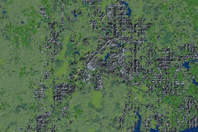
Can you see where the Orthophoto ends and the generic texturing begins?
21. Select the Render Task Mode button ![]() on the toolbar and expand the Camera category.
on the toolbar and expand the Camera category.
22. Click on the Add New Component button ![]() and when the Component Gallery opens, scroll down until you can see a component named NLCDTutorial3 Planimetric. Double-click this component to load it, and when prompted to scale its bounds to the DEM say No.
and when the Component Gallery opens, scroll down until you can see a component named NLCDTutorial3 Planimetric. Double-click this component to load it, and when prompted to scale its bounds to the DEM say No.
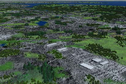
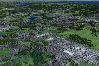
23. Right-click in an empty matrix cell select View>NLCDTutorial3 Planimetric from the popup menu. Do a preview render and you should see the following:
I’ll give you a hint – the orthophoto area is right in the center of the image, but it is virtually impossible to see where it starts and the generic texturing ends.
24. One more change to make and then we are going to finish our project by saving it as a version with modified texturing embedded. Let’s return to the NLCDTutorial1 Camera view and add some warehouses where they are clearly visible in the bottom right of the view. For this, we are going to use the Walls feature of VNS. Walls need to be defined by vectors – we can digitize these vectors by hand, in one of 3 ways:
- In an OpenGL view
- On a rendered preview of any size
- On the image preview of our orthophoto, obtained by double clicking on the image thumbnail in the Image Object Library, (or almost anywhere else in the interface where you see the thumbnail).
The first method is the least accurate, and I would advise you to use one of the other two for most hand-digitizing of vectors. The last option is a little known feature of VNS and only works when the image is georeferenced (as ours is).
The other way of creating these vectors would be to import them through the import wizard. In order to save time (and because vector digitizing is not the focus of this tutorial) the vector files for the warehouses have already been provided for you on your CD in the form of Arc Shapefiles. In addition, the elevation of the vector points has been added as an Elevation attribute to these files, allowing you to easily position them at the correct height above the ground.
25. Select File>Import Wizard from the main menu.
26. When the file requester appears, locate the Warehouses.shp file on your CD. It should be in a folder called Support Files. Select any one of the 3 shapefile files: Warehouses.shp, Warehouses.dbf or Warehouses.shx and click Open.
27. The Import Wizard should run and inform you that the file ‘Warehouses.shp’ was identified as an Arc Shapefile. Click Next and click on the Render Enabled checkbox to deselect it. We only want these vectors to place the walls of our warehouses, we don’t want them to render.
28. Click Next twice and the Import Wizard will prompt you for which coordinate system to use. It will draw this information from the shapefiles and use Custom. This is in fact the coordinate system that was set up when we imported our USGS DEMs and is based on WGS 72. Close the Coordinate System Editor and click Next.
29. On the next page of the Import Wizard, all you want to leave selected are the 3 checkboxes marked Positive E Longitude, Assign Elevations from an Attribute Field, and Load Attributes. Click Import.
30. The Import Wizard will prompt you to select which attribute fields we would like to import. Select Elevation and click OK.
31. The Import Wizard will then prompt you to select from which attribute field we would like to read our elevation values – again select Elevation, and click OK.
32. The shapefiles should load, and you should see a number of vectors appear in the bottom right foreground of the NLCDTutorial2 Camera view.
33. Now we just need to attach those vectors to our wall, and we should have some warehouses! To save some time, a pre-built Wall component suitable for our needs has been provided on the CD. Like the camera components we have already loaded, it should have been installed to your WCSContent: folder.
34. Click on the 3D Object Task Mode ![]() button on the toolbar. Select the Walls category and click the Add New Component button
button on the toolbar. Select the Walls category and click the Add New Component button ![]() above the Scene-At-A-Glance.
above the Scene-At-A-Glance.
35. The Component Gallery should open and you should see a Walls component labeled Warehouses. Double-click on it to load it into our project. Click OK when informed that the component has loaded properly and close the Walls Editor.
36. Now we have to attach the vectors we imported earlier to the Walls component we have just loaded, and the job is done. The easiest way of attaching multiple vectors to an effect is either by using search queries and dynamic linkage, or, as we shall do in this case, hard linking the vectors to the effect through the Component Library.
37. Click on the Component Library button ![]() . When the library window opens, click the Database button
. When the library window opens, click the Database button ![]() on the left to open the Database Editor. Position the editors onscreen so you can see the contents of both.
on the left to open the Database Editor. Position the editors onscreen so you can see the contents of both.
38. In the Database Editor, click and drag to select all the warehouse vectors. In the Component Library, scroll down in the Current Project Components list until you find our wall component. It should be listed between Environments and Foliage Effects. Click on it to select it.
39. Click on the Attach button ![]() to the left of the Current Project Components list. You should see a small + appear to the left of our Walls component in the library, showing that at least one vector file is attached to that component. Close both the Component Library and the Database Editor.
to the left of the Current Project Components list. You should see a small + appear to the left of our Walls component in the library, showing that at least one vector file is attached to that component. Close both the Component Library and the Database Editor.
40. Select the NLCDTutorial2 Camera View and render a preview. You should see something like this:

Great stuff! I think you will agree that our project has really progressed from our initial generic renderings, and that the techniques used to reach this point have not exactly been rocket science! All that remains for us to do is to embed the changes we have made into our project file, so that on future reloads, the template ecosystems to not take precedence over our texture changes.
41. If necessary, click on the Land Cover Task Mode button ![]() above the Scene-At-A-Glance and expand the Ecosystems category.
above the Scene-At-A-Glance and expand the Ecosystems category.
42. Double-click on the NLCD 21 Low Intensity Residential (Templated) ecosystem to open its editor.
43. Click the Embed Templated Component into Project button ![]() on the right-hand edge of the editor.
on the right-hand edge of the editor.
44. When warned that the button will disappear if you proceed with the embedding, click OK. As predicted, the button disappears, and the name of our component changes from NLCD 21 Low Intensity Residential (Templated) to NLCD 21 Low Intensity Residential.
45. Click the Next Component of Same Type button ![]() to proceed to the NLCD 22 High Intensity Residential (Templated) Ecosystem Editor.
to proceed to the NLCD 22 High Intensity Residential (Templated) Ecosystem Editor.
46. Click the Embed Templated Component into Project button ![]() on the right-hand edge of the editor.
on the right-hand edge of the editor.
47. When warned that the button will disappear if you proceed with the embedding, click OK. As predicted, the button disappears, and the name of our component changes from NLCD 22 High Intensity Residential (Templated) to NLCD 22 High Intensity Residential.
48. Click the Next Component of Same Type button ![]() to proceed to the NLCD 23 Commercial Industrial Transportation (Templated) ecosystem editor.
to proceed to the NLCD 23 Commercial Industrial Transportation (Templated) ecosystem editor.
49. Click the Embed Templated Component into Project button ![]() on the right-hand edge of the editor.
on the right-hand edge of the editor.
50. When warned that the button will disappear if you proceed with the embedding, click OK. As predicted, the button disappears, and the name of our component changes from NLCD 23 Commercial Industrial Transportation (Templated) to NLCD 23 Commercial Industrial Transportation.
51. Save your project. Close VNS and reopen it, then load your re-saved NLCDTutorial3.proj file. You should notice that the urban ecosystems have retained the changes we made to texturing and the like, while the other ecosystems are being loaded from the template project file. This allows us to create a series of projects using the NLCD template, but furnish each one with area-specific data that we may have. This gives us the best combination of speed and ease of use, allowing visualizations to be created much faster and more simply than before.
That just about wraps it up for this tutorial series. However there is one issue that needs to be noted: We have been using the Rhode Island dataset, since it is the smallest. Some of the other images are very large indeed – the GeoTIFF for Colorado is 345Mb in size! What if you only wanted to visualize a very small area of Colorado? The memory overhead of using the NLCD colormap for the whole of Colorado would be prohibitive. In the final part of the tutorial therefore, it is important that we look at ways in which you can edit the files to use only that section you want, whilst not losing the embedded georeferencing information.