3DNature

3D Landscape Design & Visualization Software published and supported by AlphaPixel

Menu

Part 3C. Downsampling Terrain

A topographic map with green, orange, and gray elevations. A crosshair marks a central location.
Getting Started with VNS 3: Terrain Basics

Part 3C. Downsampling Terrain

1. 10-meter data is great for low level scenes like the Main camera view, but what about aerial flybys higher up? We don’t need the extra terrain detail and render-time cost that comes with the higher resolution terrain. 90-m data would be more than adequate for such an application. We could download and import USGS 90-m data, but we already have a single 10-meter DEM that we can import and resample at whatever resolution we choose.

2. Launch the Import Wizard and select the original YNP-10m.elev file.

A computer dialog box showing a list of "YNP-10m.elev" files available for import. The file "YNP-10m.elev" is highlighted. There are buttons for "Open" and "Cancel" at the bottom right.

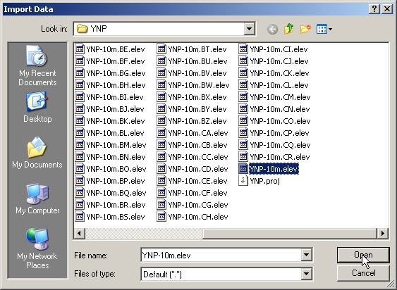
3. It will be correctly identified as a WCS/VNS DEM.

Dialog box displaying a message about a file ('YNP-10m.elev') identified as a WCS/VNS DEM, with an option to override the file type. Buttons for "Back," "Next," and "Cancel" are visible.

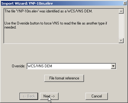
4. Click Next twice to the OUTPUT FILE TYPE AND NAME page and change the name to YNP-100m.

A software window displaying the Import Wizard for output file type and name settings. Options include "Output Format", "Name", and a checkbox labeled "Rem Import when Project Loads". The cursor is over "Next".

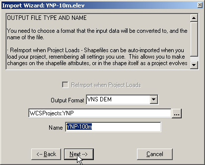
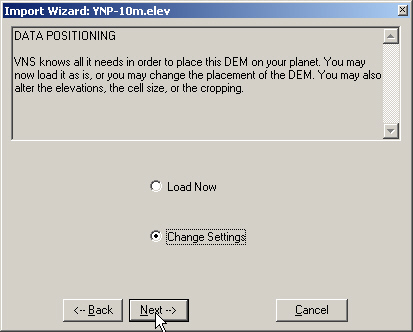
5. Click Next twice more to the DATA POSITIONING page and select Change Settings.

Screenshot of Import Wizard window titled "YNP-10m.elev" with options to "Load Now" or "Change Settings". Buttons available are "", and "Cancel".

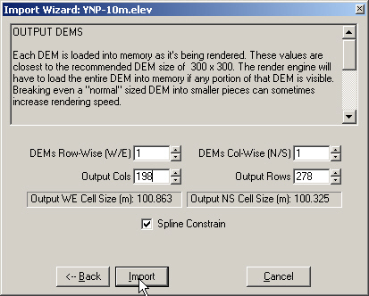
6. Click Next until you get to the OUTPUT DEMs page. This time we’re going to reduce the Output Columns and Output Rows to increase DEM cell size. We’d like cell dimensions of approximately 100 by 100 meters. Reduce the Output Columns and Output Rows values by a factor of 10 by removing the last digit from each one. The Output Cell Sizes will refresh to give us the new values. Import the data.

Screenshot of an Import Wizard window for loading DEM data. It includes DEM row and column values, output resolutions, size calculations, and an option to apply a spline constraint before importing.

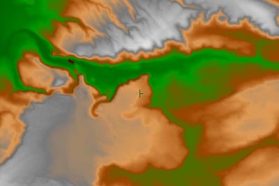
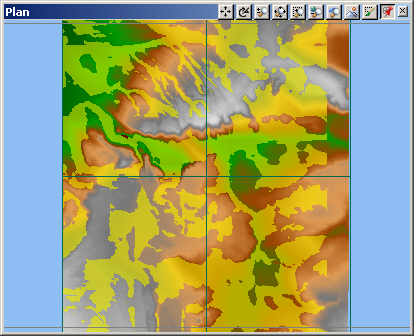
7. The realtime Plan view changed after the DEM was imported. That’s because we now have a 100-meter DEM covering the same area as the 10-meter DEMs.

A computer screen shows a topographic map with areas in green, yellow, and brown, divided into four quadrants. Various zoom and adjustment tools are visible in the toolbar at the top.

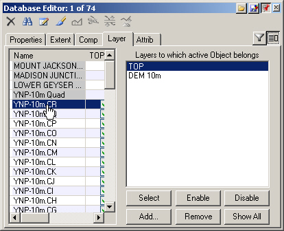
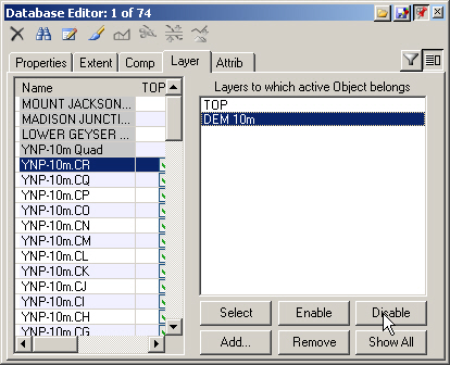
8. Let’s see how the new 100-meter DEM compares to the 10-meter DEMs. Select any YNP-10m DEM in the Database Objects list.

A database editor interface showing a list of layers and active objects, including entries like YNP-10m.CR, and categories such as TOP selected in the "Layers to which active Object belongs" section.

9. Select the DEM 10m layer and Disable.

A screenshot of the Database Editor software window showing a list of layers and options to enable or disable selected layers. The cursor is on the "Disable" button.

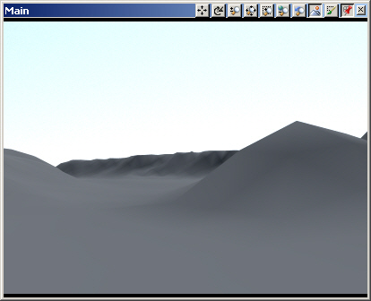
10. Open another Main view in the upper right quad. Save the project and render a preview.

A computer-generated image showing a 3D landscape with rolling hills and a clear sky, displayed in the "Main" window of a software interface.

11. The lower resolution DEM renders much faster with a lower level of terrain detail.

Scroll to top
Skip to content